De-mystifying the black box by building a working algorithm with basic Python

By Steven Chase
As a beginner Data Scientist or as an outsider looking in, Machine Learning can seem like a mystical arena. Terms like KNN, XGBoost, DBSCAN Clustering and Random Forest are enough to intimidate beginners from even peaking under the hood. But why do you even need to look under the hood? You don’t need to know exactly what these models do as long as you know how to use them, right? These models are magical black boxes anyhow. You simply put in the data that you have, and poof, the black box predicts the unknown. However, I am here to pop the hood and explain how at least one of these, K Nearest Neighbors, black boxes work. Because at the end of the day, a knowledgeable operator of these models will produce more informed and subsequently far superior predictions.
K Nearest Neighbors
K Nearest Neighbors (KNN) is a supervised machine learning algorithm. While it is most commonly used for classification, KNN can also be used for regression problems. The basic intuition behind KNN can be understood by looking at its name, K Nearest Neighbors. While trying to decide how to classify an observation, the KNN model will look for the most similar (nearest neighbor) observations in the training dataset. The K is just an input from the user that tells the model how many nearest neighbors to look for. For example, let’s say you have a car in a garage. I have to guess whether it is a truck, SUV or sedan. You won’t tell me which type it is, but I can ask you to point out the five (my k value) most similar (nearest neighbors) cars in the adjacent parking lot. Based on the types of cars you tell me are the most similar, I can make an educated guess as to the type of car in the garage. If four of the similar cars you choose are sedans and one is an SUV, I would predict that the car in the garage is a sedan. This is exactly how a KNN model works.
Now that you have a grasp of the concept, let’s dive into the algorithm and the mathematics that make this concept work.
Theory Behind KNN
As stated above, K Nearest Neighbors makes predictions based off of the most similar observations in its training data. While it can be very powerful, its predictive capability is limited to observations that are similar to the training data it has in memory. Unlike most other models, KNN does not ‘learn’ from its training dataset. Instead it holds the entire training set in memory and then compares the new observation to its stored data. In this regard, KNN is known as a ‘lazy’ model because it performs no work until a prediction is required.
When a prediction is required it does exactly what its name says. The model examines the new observation and finds the k number of most similar records (nearest neighbors) that it holds in its training set. It then makes a prediction by either returning the most common outcome of the nearest neighbors (classification) or by taking the average outcome of the nearest neighbors (regression).
Some Important Notes on Using KNN
- KNN is a simple model to implement, but as a result it is limited in the types of data it can take as input. When working with KNN, the phrase “garbage in, garbage out” is never more accurate. KNN does not handle categorical variables well so everything must be pre-processed to include numerical values only.
- Additionally, as you will see in the next section, the nearest neighbors are found by calculating the distances between the new observation and the records held in memory. Those with the smallest distances are considered most similar. Intuitively, you should understand the importance of scaling your data (so that they are all being measured on the same metric) before running a KNN model. If the data points are not measured on the same scale, a measurement of their distances will not be comparable.
Our exploration of K Nearest Neighbors will come in two parts. Part A will walk you through creating the KNN algorithm from scratch. Part B will tackle a popular classification problem. We will use both the KNN algorithm that we created as well as Scikit-Learn’s KNeighborsClassifier model to show that our algorithm is just as proficient as a popular library’s black box version.
Part A: Algorithm Implementation
Now that we understand the theory behind KNN, we can implement our own algorithm by hand in three steps.
Step 1. Calculate Euclidean distance
Step 2. Get K Nearest Neighbors
Step 3. Make predictions and determine their accuracy
Step 1: Calculate Euclidean Distance
The formula for Euclidean distance is:
Euclidean distance may sound complicated and the formula may look intimidating, but the concept is actually fairly simple. Euclidean distance is the ordinary straight-line distance between two points. The formula can be derived from the Pythagorean formula:
Where c is the Euclidean distance between data points a and b.
Let’s say that data points a and b are 2-dimensional and described by their x and y coordinates:
and
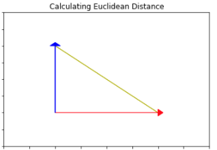
To help with understanding we can view this on a graph. On the graph below data points a and b have been plotted (represented by the large arrowheads). The Euclidean distance we are trying to calculate is the vector drawn in yellow.
By drawing in the vectors representing the data points (in blue and red) we can clearly see that the yellow Euclidean distance is the hypotenuse of the triangle.
We know that the length of the vectors for point a and b can be calculated by and
So it follows that,
This is the basic formula for Euclidean distance for 2-D datapoints.
However, this can be expanded to 3-D and beyond:
More succintly written as,
Which is the finalized formula of Euclidean distance we saw above.
Given our understanding of the mathematics behind calculating the Euclidean distance, how can we write that calculation in Python?
When working with datasets, each row is a data point. Each column represents another feature or dimension of the data point. The subject of dimensionality and furthermore the curse of dimensionality is outside the scope of this article but is a crucial concept to understand when building your own machine learning models. For the purposes of this article, I will leave further research of that topic to you.
To calculate the Euclidean distance between two points we can use the following function:
# Helper method to calculate the square root
def sq_rt(x):
  return x** 0.5

# Calculate the Euclidean distance between two vectors (data points)
def euclidean_distance(row_1, row_2):
  # Create a distance variable to save sum of calculations to
  distance = 0.0
  # Iterate through each column of the row
  # Except for the last column which is where the target variable is stored
  for i in range(len(row_1)-1):
    # Calculate the length vectors for each dimension and sum them
    distance += (row_1[i]- row_2[i])**2
  # Return the square root of the sum of the distances
  return sq_rt(distance)
The function above assumes that the output target is the last column of the row and is therefore not included in the distance calculations. In our final KNN class we will have a fit method that saves the X values and the target separately and this function will be modified slightly.
Step 2: Get K Nearest Neighbors
Now that we know how to calculate the distance between two data points, we can find the K Nearest Neighbors (closest instances in the training data) to our new data point.
First, we can use the above function to calculate the distances between our new observation and each data point in our training set. Once calculated, we can return the k number of instances with the smallest distances from our new data point.
The below function get_KNN() will implement this idea in Python.
# Return the K Nearest Neighbors to the new observation

# Input is the training data, test observation, and the number of neighbors (k) to return
def get_KNN(train, test_row, k):
  # Save the rows and calculated distances in a tuple
  distances = list()

  # Iterate through each row in the training data
  # Use the Euclidean distance function to calculate the distances between the train row and the new observation
  for train_row in train:
    euc_dist = euclidean_distance(test_row, train_row)
    # Save the row and calculated distance
    distances.append((train_row, euc_dist))

  # Sort by using the calculated distances (the second item in the tuple)
  distances.sort(key= lambda tup: tup[1])

  # Populate a list with K Nearest Neighbors
  n_neighbors = list()

  # Get the nearest k neighbors by returning the k first instances in the sorted distances list
  # Return just the first value in the tuple (the row information)
  for i in range(k):
    n_neighbors.append(distances[i][0])

  # Return the list of nearest neighbors
  return n_neighbors
Step 3A: Make Predictions
We have used our knowledge of Euclidean distance to find the K Nearest Neighbors to our test data point. Now we can get to the power of the algorithm, making predictions.
Intuitively, by looking at the outputs of our nearest neighbors, we should be able to predict an output for our test case.
Classification: For a classification problem, our prediction will be whichever output occurs most frequently among the nearest neighbors.
The function below utilizes the output from the get_KNN() function to implement the idea of classification prediction:
# Make a classification prediction with k Nearest Neighbors
def predict_classification(train, test_row, k):
  # Find the nearest neighbors
  n_neighbors = get_KNN(train, test_row, k)

  # Populate a list with the target output (the last column) from each KNN row
  output_values = [row[-1] for row in n_neighbors]

  # Make prediction by counting each occurrence of output values
  # Return the output value that occurs the most frequently
  prediction = max(set(output_values), key= output_values.count)
  # Return the prediction
  return prediction
Regression: For a regression problem, we use the same logic of looking at the output values of the K Nearest Neighbors. Instead of returning the most common occurrence as our prediction, we will return the mean value of the nearest neighbors’ outputs. The function below utilizes the output from the get_KNN() function to make a regression prediction.
# Make a regression prediction with K Nearest Neighbors
def predict_regression(train, test_row, k):
  # Find the nearest neighbors
  n_neighbors = get_KNN(train, test_row, k)

  # Populate a list with the target output (the last column) from each KNN row
  output_values = [row[-1] for row in n_neighbors]

  # Make prediction by calculating the mean of the output values from the nearest neighbors
  prediction = sum(output_values) / len(output_values)
  # Return the prediction
  return prediction
For ease of understanding, we created the above functions examining only one new data point. Generally, we are not looking for a single prediction, but instead, a prediction for each point in a larger dataset. To adapt the above functions to handle multiple predictions, iterate through your new dataset, calling the predict function on each new point.
This is implemented for classification predictions in the function below.
# Create predictions for multiple new data points, classification

def multiple_classifications(train, test, k):
  # Create a list to hold all of the predictions
	predictions = list()

  # For each row in the test data, call the predict function
  for row in test:
		predicted_output = predict_classification(train, row, k)
		predictions.append(predicted_output)

  # Return the populated list of predictions
  return predictions
The predict_regression() function can also be similarly modified to handle multiple regression predictions.
Step 3B: Determine Accuracy of Predictions
We may have predictions but what use are they if we do not know how accurate they are?
Classification error metric: For classification, we will use accuracy to determine the strength of our predictive model.
This can be calculated by dividing the number of correct predictions by the total amount of predictions the model makes.
accuracy = correct_predictions / total_predictions
A Python function for this can be implemented as follows:
# Return accuracy by comparing predicted output to the known actual output

def model_accuracy(predicted, actual):

    # Compare each prediction to the known test output
    predict_bool = [predicted[i] == actual[i] for i in range(len(predictions))]

    # Return the percentage of correct predictions
    accuracy = sum(predict_bool) / len(self.y_test)
    return accuracy
Regression error metric: For regression there are a few choices of error metrics to evaluate your model’s ability: mean squared error, root mean squared error, mean absolute error, and . Explaining each one is outside the scope of this article, but I suggest you spend some time learning the pros and cons for each one. For our example, we will use mean squared error (MSE) as our error metric.
Calculating the MSE is the average of the squared differences between the actual output and the predicted output.
Mathematically, this formula can be written as:
MSE =
In Python, we can implement an MSE calculation function as follows:
# Return the mean square error by comparing the predicted outputs with the known outputs

def model_mse(predicted, actual):
    # Start a mse variable at 0
    mse = 0

    # For each predicted value - square the difference between the actual and predicted output
    # Sum them all and divide by the number of predicted outputs
    for i in range(len(predicted)):
      mse += (actual[i] - predicted[i])**2
      mse = mse / len(predicted)

    # Return the calculated mean square root
    return mse
Put the pieces together in a KNN class
Now that we have all of the pieces, we can wrap them all in a K Nearest Neighbor class. All of the functions defined and explained above will be methods that you can call on the class.
- note that while all of the concepts from the functions above are the same, the methods have been modified slightly to fit the class implementation
# K Nearest Neighbors Class
'''
Class is initialized by setting k (number of nearest neighbors you want to look at)
Then call the .fit() method to save the X_train matrix and y_train vector
The method .predict_classification() will return classification predictions given X_test
The method .predict_regression() will return regression predictions given X_test
'''

class KNN():
  def __init__(self, k=3):
    # k is number of nearest neighbors to return, default is 3
    self.k = k


  def sq_rt(self, x):
    '''
    Helper method to return the square root.
    To be used in Euclidean distance calculations.
    '''
    return x**0.5

  def euclidean_distance(self, row_1, row_2):
    '''
    Helper method to calculate the Euclidean distance between two points
    To be used in get_KNN to calculate the closest training points to the test data.
    '''
    # Save a distance variable to save sum of calculations to
    distance = 0.0
    # Iterate through each column of the row
    for i in range(len(row_1)):
      # Calculate the length vectors for each dimension and sum them
      distance += (row_1[i]- row_2[i])**2
    # Return the square root of the sum of the distances
    return self.sq_rt(distance)

  def fit(self, X_train, y_train):
    '''
    Our algorithm needs the input data to be a python list
    Fit method will convert y_train to a list and save both y_train and X_train to memory
    X_train will already be converted to a list during the scaling process
    '''
    self.X_train = X_train
    self.y_train = y_train.values.tolist()

  def get_KNN(self, test_row):
    '''
    Helper method for prediction methods.
    Will take in one test row and calculate the K Nearest Neighbors.
    Returns a list of nearest neighbors.
    '''

    # Save the rows and calculated distances in a tuple
    distances = list()

    # Iterate through each row in the training data
    for i in range(len(self.X_train)):
      # Use the Euclidean distance function to calculate the distances between the train row and the new observation
      euc_dist = self.euclidean_distance(test_row, self.X_train[i])
      # Save the index (to later recall the output value), the row data and the calculated distance
      distances.append((i, self.X_train[i], euc_dist))


    # Sort by using the calculated distances (the third item in the tuple)
    distances.sort(key= lambda tup: tup[2])

    # Populate a list with K Nearest Neighbors
    n_neighbors = list()

    # Get the nearest k neighbors by returning the k first instances in the sorted distances list
    # Return just the first value in the tuple (the row information)
    for i in range(self.k):
      n_neighbors.append(distances[i][:2])

    # Return the list of nearest neighbors
    # Don't need to save it to self because we are just using it to populate a list
    # Used for the prediction method.
    # The prediction method will save the important information
    return n_neighbors

  def helper_predict_classification(self, test_row):
    '''
    Method returns a classification prediction for a single given test data point.
    This method will be utilized in the predict_classification method which will be
    capable of making predictions for a large X_test dataset.
    '''

    # Find the nearest neighbors
    n_neighbors = self.get_KNN(test_row)

    # Use the index values of the nearest neighbors to recall their target outputs

    # Store the index values of the n_neighbors
    train_output = [n_neighbors[i][0] for i in range(self.k)]

    # Use the index values from the n_neighbors to return their associated outputs from y_train
    output_values = [self.y_train[value] for value in train_output]

    # Make a prediction by counting each occurrence of output values
    # Return the output value that occurs the most frequently
    prediction = max(set(output_values), key= output_values.count)
    # Return the prediction
    return prediction

  def predict_classification(self, X_test):
    '''
    Method utilizes the helper_predict_classification to return predictions for
    multiple test rows stored in X_test.
    '''
    # Save X_test to memory
    self.X_test = X_test

    # Create a list to hold all of the predictions
    self.predictions = []

    # For each row in X_test, call the predict_classification helper method
    for test_row in self.X_test:
      predicted_output = self.helper_predict_classification(test_row)

      # Save the prediction for each row in X_test
      self.predictions.append(predicted_output)

    # Return the list of predictions for each datapoint in X_test
    return self.predictions

  def helper_predict_regression(self, test_row):
    '''
    Method returns a regression prediction for a single given test data point.
    This method will be utilized in the predict_classification method which will be
    capable of making predictions for a large X_test dataset.
    '''

    # Find the nearest neighbors
    n_neighbors = self.get_KNN(test_row)

    # Use the index values of the nearest neighbors to recall their target outputs

    # Store the index values of the n_neighbors
    train_output = [n_neighbors[i][0] for i in range(self.k)]

    # Use the index values from the n_neighbors to return their associated outputs from y_train
    output_values = [self.y_train[value] for value in train_output]

    # Make prediction by calculating the mean of the output values from the nearest neighbors
    prediction = sum(output_values) / len(output_values)

    # Return the prediction
    return prediction

  def predict_regression(self, X_test):
    '''
    Method utilizes the helper_predict_classification to return predictions for
    multiple test rows stored in X_test.
    '''
    # Save X_test to memory
    self.X_test = X_test

    # Create a list to hold all of the predictions
    self.predictions = []

    # For each row in X_test, call the predict_classification helper method
    for test_row in self.X_test:
      predicted_output = self.helper_predict_regression(test_row)

      # Save the prediction for each row in X_test
      self.predictions.append(predicted_output)

    # Return the list of predictions for each datapoint in X_test
    return self.predictions

  def model_accuracy(self, y_test):
    '''
    Calculates the accuracy of the model's classification predictions.
    Compares the predicted output values with the known test output values.
    '''
    # y_test must be a python list
    # Method will convert the input to python lists and save it in memory
    self.y_test = y_test.values.tolist()

    # Compare each prediction to the known test output
    predict_bool = [self.predictions[i] == self.y_test[i] for i in range(len(self.predictions))]

    # Return the percentage of correct predictions
    return sum(predict_bool) / len(self.y_test)

  def model_MSE(self, y_test):
    '''
    Calculates the mean squared error of the model's regression predictions.
    Calculated by summing all of the squares of the differences between actual
    and predicted, and then dividing by the number of observations.
    '''
    # y_test must be a python list
    # Method will convert the input to python lists and save it in memory
    self.y_test = y_test.values.tolist()

    # Start a mse variable at 0
    mse = 0

    # For each predicted value - square the difference between the actual and predicted output
    # Sum them all and return divide by the number of predicted outputs
    for i in range(len(self.predictions)):
      mse += (self.y_test[i] - self.predictions[i])**2
      self.mse = mse / len(self.predictions)

    # Return the calculated mean square root
    return self.mse
Comparing Scikit-Learn’s KNN with our own KNN algorithm
Let’s see how our algorithm compares to Scikit-Learn’s KNN implementation.
Titanic Dataset
We will only work with classification. After following along with this article, try to implement a regression problem with the same KNN class we created.
We will work with a very common and easily accessible dataset to make it easier for readers to follow along. The Titanic dataset is one of the most popular datasets for beginning to learn classification models. The data is already cleaned and has a clear classification target of ‘survived’ or ‘did not survive’. After only a few basic pre-processing steps, we will have a perfect dataset for our KNN models.
Download your own copy of the Titanic dataset and follow along!
In order to implement either model, we need to first pre-process the Titanic data. As mentioned before, KNN only handles numeric data and that data must be scaled to make them comparable.
After downloading the Titanic csv and loading it into your notebook, (for instructions look at my source code here) we can look at the first few records to understand the features of the data we are working with.
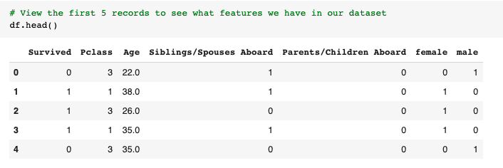
The first column ‘Survived’ is our target. We are trying to predict whether the passenger survived (1) or did not (0). The remaining columns are features we can choose from to use to predict our target. In order to make the pre-processing easier and consistent across all segments of our data, we will make a pre-processing function.
The function will drop two categories: ‘Name’ and ‘Fare’. The ‘name’ category will get dropped because a passenger’s survival rate doesn’t depend on their name and the ‘Fare’ category will get dropped because it is directly tied to ‘Pclass’ and is therefore redundant. The last task we have in pre-processing is to convert the ‘Sex’ column into numerical values. We can accomplish this by using pandas’ get_dummies() method to One-Hot-Encode the ‘Sex’ column so that there is a column for ‘male’ and ‘female’ populated by 1’s and 0’s.
# Build a pre-processing function that will clean the data for use in our KNN models

def pre_process(df):
  # Make a copy of the data
  df = df.copy()

  # Drop Name because target does not depend on name
  # Drop Fare because it is directly tied to Pclass and therefore redundant information
  df = df.drop(['Name', 'Fare'], axis=1)

  # One-Hot-Encode the sex column using pd.get_dummies()
  dummies = pd.get_dummies(df['Sex'])
  # Add the new 'male' and 'female' columns to the existing df and drop the original 'Sex' column
  df = pd.concat([df, dummies], axis= 'columns').drop('Sex', axis= 'columns')

  # Return the pre-processed df
  return df
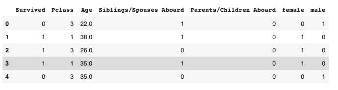
Now we can use the pre-process function to format the Titanic dataset in the way that KNN needs it to be.
# Run pre-process function and view returned df

df = pre_process(df)
df.head()
As we can see, the data is now in the proper format for our KNN models; all values are numeric and there are no redundant columns.
Now that our data has been pre-processed, we can separate the target from the features. Our target is ‘Survived’ and our features are all of the columns except for ‘Survived’.
# Define target and features
features = df.columns.drop('Survived')
target = 'Survived'

# Create feature matrix and target vector
X = df[features]
y = df[target]
In order to test our algorithms, we need to set aside some of the data we have. This is standard practice for supervised machine learning models. We will use 80% of our data to train our model, and the remaining 20% will be used to test the performance of our model.
Thankfully, Scikit-Learn has a function to do this for us.
# Import train-test split
from sklearn.model_selection import train_test_split

# Split the df into 80% train 20% test data
X_train, X_test, y_train, y_test = train_test_split(X, y, test_size= 0.20, random_state=42)
Our data has been cleaned and the target and features have been separated and split into training and testing datasets. We have one last pre-processing step to take before being able to run our data: scaling. As we mentioned before, KNN makes predictions based on distances between data points. As such, it is crucial that all of the data it is comparing is on the same scale. In our Titanic dataset, most of the data has a maximum value of 3 or under. However, the ‘Age’ column has a maximum value of 80. This difference in magnitude will lead to less optimized results from KNN. To solve this we will use one of scikit-learn’s scaling packages, Normalizer.
Normalizing in scikit-learn rescales each observation to have a length of 1. We are using this particular method because it is useful for sparse datasets, meaning lots of zeros, which our dataset has. When scaling your data, you want to fit and transform on your training data, and only transform your testing data. Fitting the scaler to your test data will result in data leakage.
# Normalize Data

# Import Normalizer
from sklearn.preprocessing import Normalizer

# Instantiate scaler model
scaler = Normalizer()

# Fit and Transform X_train
X_train = scaler.fit_transform(X_train)

# Transform X_test
X_test = scaler.transform(X_test)
If you’ve stuck with us this far, it’s about to pay off. Let’s run some KNN models!
Baseline Accuracy
When evaluating model performance, we want to start with a baseline accuracy. This is the accuracy score for if we were to guess the majority outcome every time. It gives us a starting point to compare our models to. The baseline metric is the best we can do without models. Hopefully, our models can improve over the baseline.
# Find the majority count
y_train.value_counts()
0    434
1    275
Name: Survived, dtype: int64
This shows us that the majority of the passengers in the training data did not survive. (434 did not survive (0), 275 did survive (1))
We run the same code above to get the count of survived and didn’t survive for our y_test targets. (111 did not survive (0), 67 did survive (1))
# Survival counts for y_test
y_test.value_counts()
0    111
1     67
Name: Survived, dtype: int64
If we were to guess the majority, that the passenger did not survive (0), for every test case we would get 111 correct out of 178 total test cases.
111/178 = 0.624
That gives us a baseline accuracy of 62.4%.
Titanic Predictions Using Scikit-Learn’s KNeighborsClassifier
Let’s start by making predictions and calculating the accuracy of Scikit-Learn’s KNeighborsClassifier model.
This can be done by the following steps:
- Instantiate the model
- Fit the model with our training data
- Make predictions based off of our test features
- Provide the known test targets to determine the accuracy
# Import the model
from sklearn.neighbors import KNeighborsClassifier

# Instantiate the KNClassifier object
scikit_KNN = KNeighborsClassifier(n_neighbors=3)

# Fit the model with training data
scikit_KNN.fit(X_train, y_train)

# Make predictions
print(scikit_KNN.predict(X_test))

# Calculate accuracy
scikit_KNN.score(X_test, y_test)
Our prediction array is:
[0 0 0 0 0 1 0 0 0 0 1 1 1 0 0 0 0 1 0 0 0 1 1 0 0 0 0 0 0 1 1 0 1 0 1 0 0
 1 1 1 1 0 1 0 0 0 0 0 0 0 0 0 0 0 1 0 0 0 1 0 0 1 0 1 0 0 0 1 0 0 0 1 0 0
 0 1 1 0 1 0 0 0 0 0 1 1 0 0 0 0 1 1 0 1 0 0 0 0 1 0 0 0 0 1 0 0 0 1 0 0 1
 1 0 0 0 0 0 1 0 0 1 0 1 0 1 0 0 1 1 1 0 1 0 0 0 0 0 0 0 1 1 0 0 0 0 1 0 0
 0 0 0 1 0 0 1 1 0 1 0 0 0 1 0 0 0 1 0 1 0 0 1 1 0 0 1 1 1 0]
With an accuracy of:
0.7584269662921348
Considering the baseline accuracy was 62.4%, Scikit-Learn’s model is an improvement at 75.84%.
Titanic Predictions Using Our Own Algorithm
Let’s see how our algorithm does compared to the results from Scikit-Learn.
Our model can be implemented in the exact same way:
- Instantiate the model
- Fit the model with our training data
- Make predictions based off of our test features
- Provide the known test targets to determine the accuracy
# Make sure you run the KNN Class above to load the algorithm

# Instantiate our algorithm
our_KNN = KNN(3)

# Fit the model with training data
our_KNN.fit(X_train, y_train)

# Make predictions based off of our test features
print(our_KNN.predict_classification(X_test))

# Calculate the accuracy of our model
our_KNN.model_accuracy(y_test)
The prediction array for our algorithm is:
[0, 0, 0, 0, 0, 1, 0, 0, 0, 0, 1, 1, 1, 0, 0, 0, 0, 1, 0, 0, 0, 1, 0, 0, 0, 0, 0, 0, 0, 0, 1, 0, 1, 0, 1, 0, 1, 1, 1, 1, 1, 0, 1, 0, 0, 0, 0, 0, 0, 0, 0, 0, 0, 0, 1, 0, 0, 1, 1, 0, 0, 1, 1, 1, 0, 0, 0, 1, 0, 0, 0, 1, 0, 0, 0, 1, 1, 0, 1, 0, 0, 0, 0, 0, 1, 1, 0, 0, 0, 0, 1, 1, 0, 1, 0, 0, 0, 0, 1, 0, 0, 0, 0, 1, 0, 0, 0, 1, 0, 0, 1, 1, 0, 0, 0, 0, 0, 1, 0, 0, 1, 0, 0, 0, 1, 0, 0, 1, 1, 1, 0, 1, 0, 0, 0, 0, 0, 0, 1, 1, 1, 0, 0, 0, 0, 1, 0, 0, 0, 0, 0, 1, 0, 0, 0, 1, 0, 1, 0, 0, 0, 1, 0, 0, 0, 1, 0, 1, 0, 0, 1, 1, 0, 0, 1, 1, 1, 0]
With an accuracy of:
0.7696629213483146
Our algorithm resulted in an accuracy of 76.96%! Slightly better accuracy than Scikit-Learn’s method and far better than our baseline.
What’s Next?
We have walked through how to implement a K Nearest Neighbors machine learning algorithm that will work with either classification or regression problems. Then we walked through a classification problem using the Titanic dataset.
For further understanding and practice:
- Find your own dataset for a regression problem and use the predict_regression() method that we created in our KNN class.
- Implement a different distance metric like Manhattan distance or Hamming distance rather than Euclidean distance to calculate the nearest neighbors
- Implement different error metrics for both classification and regression
Hopefully this tutorial has removed any mystery around K Nearest Neighbors. As with all algorithms, it is firmly seated in mathematics, not magic. Having written your first algorithm by hand, you should now have the confidence to tackle any other black box model out there. True, some may be more complicated than others, but by lifting the hood and understanding the moving parts underneath, you will be able to yield much more powerful predictive models.
Resources
Brownlee, J. (2020, February 24). Develop k-Nearest Neighbors in Python From Scratch. Retrieved from Machine Learning Mastery: https://machinelearningmastery.com/tutorial-to-implement-k-nearest-neighbors-in-python-from-scratch/